4 Ways to Create a Table of Contents in Microsoft Excel

Do you need to organize all the worksheets in your Excel workbook? Are you wondering how to create a table of contents in Excel? This Excel tutorial will explain the easiest ways to create an Excel table of contents with automation.

A table of contents helps you to navigate the document when it’s too large to remember all the sections. The same can also happen with an Excel workbook. This especially happens when the Excel file contains hundreds of worksheets. These worksheets can contain PivotTables, charts, graphs, dashboards, data-entry sheets, and so on.

Instead of remembering the workbook or writing down the important worksheet names on a sticky note, you can always create a table of contents in Excel. Unfortunately, there are no built-in functions or features in Excel that let you create a table of content in a single click like Microsoft Word.

Therefore, follow along with the methods mentioned below to create your table of contents in Excel without asking for help.

Reasons to Create Excel Table of Contents

1. Simplifies the challenging task of navigating through extensive Excel workbooks. Also, an Excel table of contents is effortless to find specific sections and data points within the workbook.
2. Offers a valuable time-saving feature by granting you swift access to targeted information. Thus, sparing you from the frustration of endlessly scrolling through sheets and tabs.
3. A table of contents in Excel elevates user experience by presenting a visually pleasing and well-organized overview of the workbook’s contents.
4. You can effectively arrange data by logically grouping related sheets or sections, aiding in maintaining a structured and coherent layout for large workbook management.
5. It also provides a convenient means of swiftly referencing vital data, charts, and tables, reducing the need for time-consuming searches. Thus, you can focus on actual data analysis and visualization.
6. The end-users, data entry operators, stakeholders, or the audience can comprehend the workbook easily when there is a table of contents in the Excel file.
7. It supports collaboration and teamwork by simplifying content location. You can make it easy for team members to locate specific sections for input and review.
8. Minimizes the potential for errors by preventing accidental modifications to unrelated data when navigating through the workbook, thus ensuring data integrity.

Create an Excel Table of Contents Using A Formula

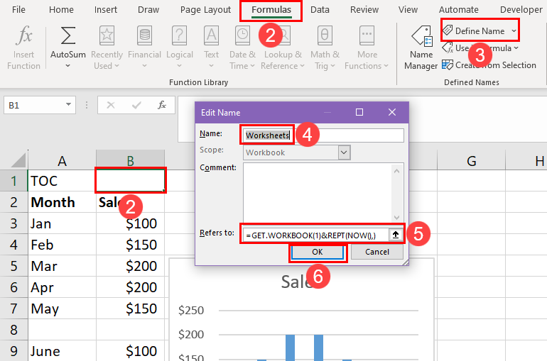
This method will utilize a formula containing a named range element. This is a semi-automatic method since you must perform a few manual tasks as well to create the table of contents for the first time.

Define a Named Range

1. Go to the first worksheet of the workbook.
2. Click any blank cell and select the Formulas tab.
3. Click the Define Name drop-down menu inside the Defined Names block.
4. On the Edit Name dialog box, enter Worksheets in the Name field.
5. Now, in the Refers to field enter the following formula:

=GET.WORKBOOK(1)&REPT(NOW(),)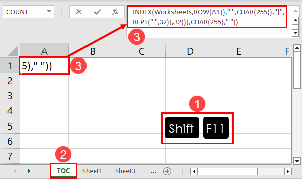

1. Click OK to close the dialog box.

Make a Table of Contents

1. Add a new worksheet tab at the beginning of all the existing tabs by pressing Shift + F11 keys.
2. Rename it to TOC.
3. Go to the cell A1 of the TOC tab and enter the following formula:

=IF(ROW(A1)>SHEETS(),REPT(NOW(),),SUBSTITUTE(HYPERLINK("#'"&TRIM(RIGHT(SUBSTITUTE(SUBSTITUTE(INDEX(Worksheets,ROW(A1))," ",CHAR(255)),"]",REPT(" ",32)),32))&"'!A1",TRIM(RIGHT(SUBSTITUTE(SUBSTITUTE(INDEX(Worksheets,ROW(A1))," ",CHAR(255)),"]",REPT(" ",32)),32))),CHAR(255)," "))

To complete the TOC, follow these steps:

1. Hit the Enter button and you should see the TOC worksheet name in the cell A1 .
2. Now, drag the fill handle down the column until you get a blank cell.
3. By now, Excel should have populated hyperlinks to all Excel worksheets in your workbook.
4. Click on any of the worksheet names to navigate to that Excel tab.

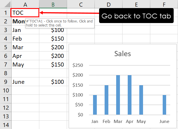
To go back to the TOC tab, simply click the worksheet name at the bottom of the Excel application. Alternatively, you can add the link to TOC in all the worksheets. To do this, either copy cell A1 from the TOC tab to all the worksheets in the workbook or use the following Excel VBA script:

Sub CopyFormulaToAllWorksheetsWithNewRowAtTop() Dim SourceSheet As Worksheet Dim DestSheet As Worksheet Dim SourceCell As Range Dim DestCell As Range Dim FirstRow As Long Dim ws As Worksheet Set SourceSheet = ThisWorkbook.Worksheets(1) Set SourceCell = SourceSheet.Range("A1") For Each ws In ThisWorkbook.Worksheets If ws.Name <> SourceSheet.Name Then Set DestSheet = ws Set DestCell = DestSheet.Range(SourceCell.Address) If DestCell.Value <> "" Then FirstRow = DestSheet.Cells(DestSheet.Rows.Count, "A").End(xlUp).Row DestSheet.Rows(FirstRow).EntireRow.Insert End If DestCell.Formula = SourceCell.Formula End If Next ws End Sub 

Refer to the Excel VBA section below to learn how to use the above VBA script in your Excel workbook.

Here are the conditions to use the above method:

• You must save the workbook as a Macro-enabled workbook or in XLSM format.
• The formula will reveal and link all the Excel worksheets in the workbook, including hidden ones.
• The Excel table of contents will reflect the following changes:
  • Additions and deletions of worksheets
  • Changing worksheet names
  • Altering the order of the worksheet tabs

  Create a Table of Contents in Excel Using Power Query

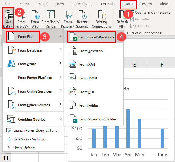
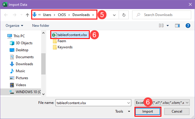
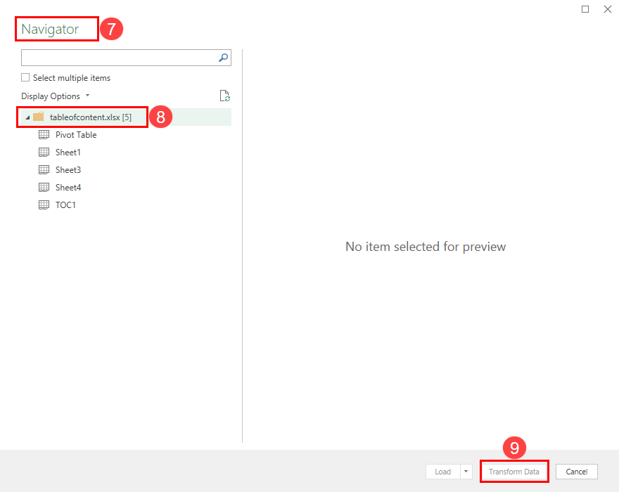
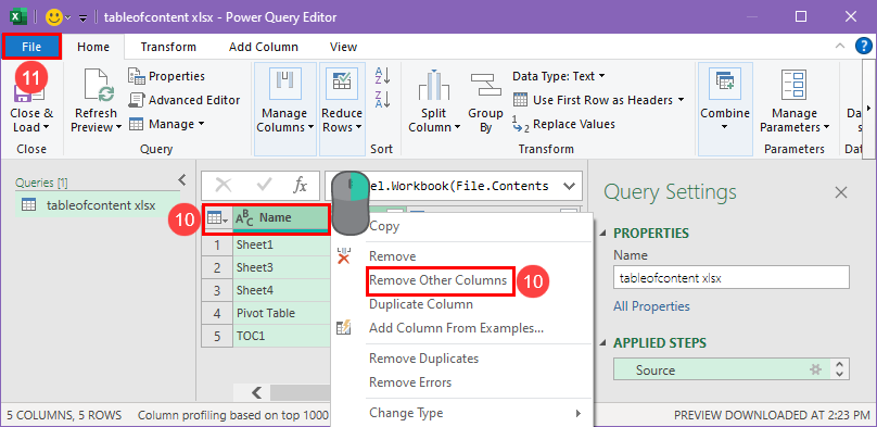
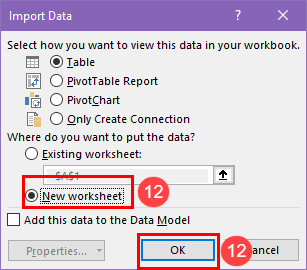
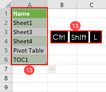
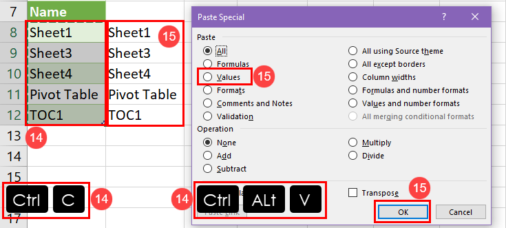
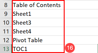
  You can use the Power Query tool to create a list of all worksheets in the workbook. Then, apply the HYPERLINK function to create an Excel table of contents quickly.

  So, if you’re accessing a large workbook using Power Query and it doesn’t have any table of contents tab, you can add that too to organize the workbook.

  Create a List of Tabs Using Power Query

  

  1. Open any Excel workbook and click the Data tab on the Excel ribbon menu.
  2. Click the Get Data button inside the Get & Transform Data block.
  3. Hover the mouse cursor over the From File option.
  4. On the overflow menu, click From Excel Workbook.
  
  1. On the Import Data dialog box, navigate to the Excel file for which you need to create a TOC.
  2. Select the file and hit the Import button.
  
  1. You should now see all the worksheets of the Excel file on the Power Query Navigator dialog box.
  2. Click the parent folder, for example, the tableofcontents.xlsx, and select the Transform Data button.
  3. The workbook will open in the Power Query Editor interface.
  
  1. Right-click the first column or the Name column and choose the Remove Other Columns option on the context menu.
  2. Click the File menu and choose Close & Load To.
  
  1. Select the New worksheet option on the Import Data window and click OK.
  
  1. Highlight the whole imported data and press Ctrl + Shift + L to remove the filters.
  
  1. Highlight the table again, press Ctrl + C to copy, select a destination cell, and press Ctrl + Alt + V to open Paste Special.
  2. On the Paste Special dialog box, choose Values, and click OK.
  
  1. Delete any unnecessary entries from the imported table.

  Make the TOC Tab

  

  1. Rename the worksheet to TOC.
  2. Write Table of Contents in the first cell: A1 .
  3. Enter the following formula into the adjacent cell to the right of the first worksheet name:

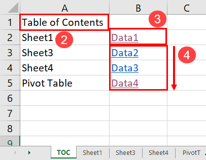
  =HYPERLINK("#Sheet1!A1","Data1")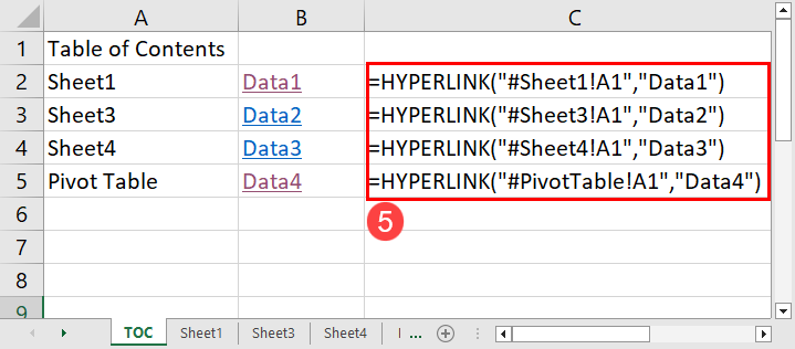

  

  1. Now, copy and paste the same formula down the column for all other worksheets.
  1. Rename formula elements like Sheet1 with the next worksheet’s name and Data1 to Data2 , and so on.

  Create a Table of Contents in Excel Using Excel VBA

  You can also use the following VBA script to add an Excel table of contents to any workbook that has many tabs, tables, PivotTables, etc.

  Excel VBA Script

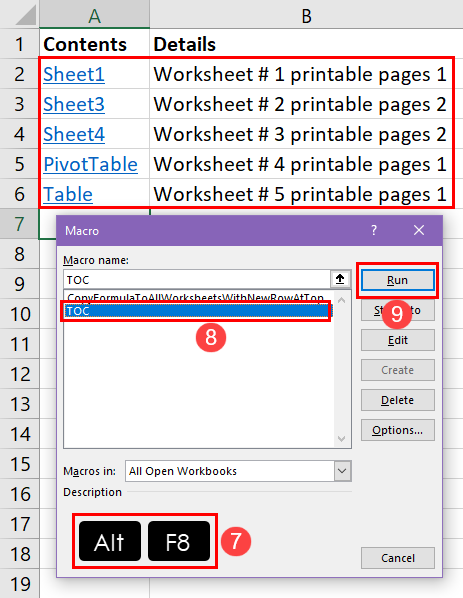
  Sub TOC() Dim TOCSheet As Worksheet Dim ws As Worksheet Dim rowNum As Long Set TOCSheet = ThisWorkbook.Sheets.Add(After:=ThisWorkbook.Sheets(ThisWorkbook.Sheets.Count)) TOCSheet.Name = "Table of Contents" TOCSheet.Cells(1, 1).Value = "Contents" TOCSheet.Cells(1, 2).Value = "Details" rowNum = 2 For Each ws In ThisWorkbook.Worksheets If ws.Name <> TOCSheet.Name Then TOCSheet.Cells(rowNum, 1).Value = ws.Name TOCSheet.Cells(rowNum, 2).Value = "Worksheet # " & ws.Index & " printable pages " & GetPrintablePageCount(ws) TOCSheet.Hyperlinks.Add _ Anchor:=TOCSheet.Cells(rowNum, 1), _ Address:="", _ SubAddress:=ws.Name & "!A1", _ TextToDisplay:=ws.Name rowNum = rowNum + 1 End If Next ws End Sub Function GetPrintablePageCount(ws As Worksheet) As Long Dim pageCount As Long pageCount = ws.PageSetup.Pages.Count GetPrintablePageCount = pageCount End Function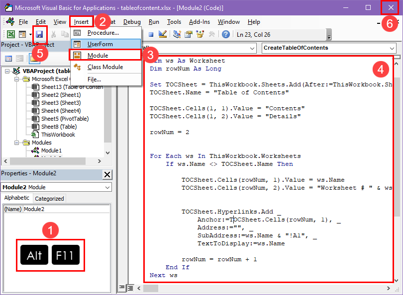

  How to Use the Code

  

  1. Click Alt + F11 to call the Excel VBA Editor.
  2. Click the Insert button on the menu bar.
  3. Choose Module in the context menu.
  4. Copy and paste the Excel VBA script mentioned above in the module.
  5. Click the Save button.
  6. Close the Excel VBA Editor.
  
  1. Hit Alt + F8 to call the Macro dialog box.
  2. Select the TOC macro.
  3. Hit the Run button to create the Excel table of contents.

  You might want to format the newly-created Table of Contents worksheet so that it becomes readable and presentable.

  Create an Excel Table of Contents Using Office Scripts

  On Excel for the web or Excel for Microsoft 365 desktop applications, you can use the Office Scripts scripting tool to create automated Excel functions, like making an Excel table of contents worksheet. Find below the steps you must follow:

  Make a List of Worksheets in a New Tab

  

  1. Click the Automate tab and click the New Script button.
  2. Into the Code Editor that shows up, copy and paste the following script:

  function main(workbook: ExcelScript.Workbook) < // Create a new worksheet called "TOC". let sheetNamesSheet = workbook.addWorksheet("TOC"); // Get the collection of worksheets in the workbook. let worksheets = workbook.getWorksheets(); // Create a string that will contain the list of sheet names. let sheetNames = ""; // Iterate over the worksheets and add their names to the string. for (let worksheet of worksheets) < sheetNames += worksheet.getName() + "\n"; >// Set the value of each cell in the "SheetNames" sheet to a sheet name. for (let i = 1; i >

  1. Click the Save script button.
  2. Hit the Run button to execute the script.

  Office Scripts will automatically create a new worksheet named TOC and list all the existing worksheets in the workbook in the order they appear.

  Add Links to the Worksheets of the TOC

  

  1. Go to the newly-created sheet or the TOC sheet.
  2. You must see the full list of worksheets in the workbook.
  3. Click Automate and select the New Script option.
  4. Inside the Code Editor, copy and paste this Office Scripts code:

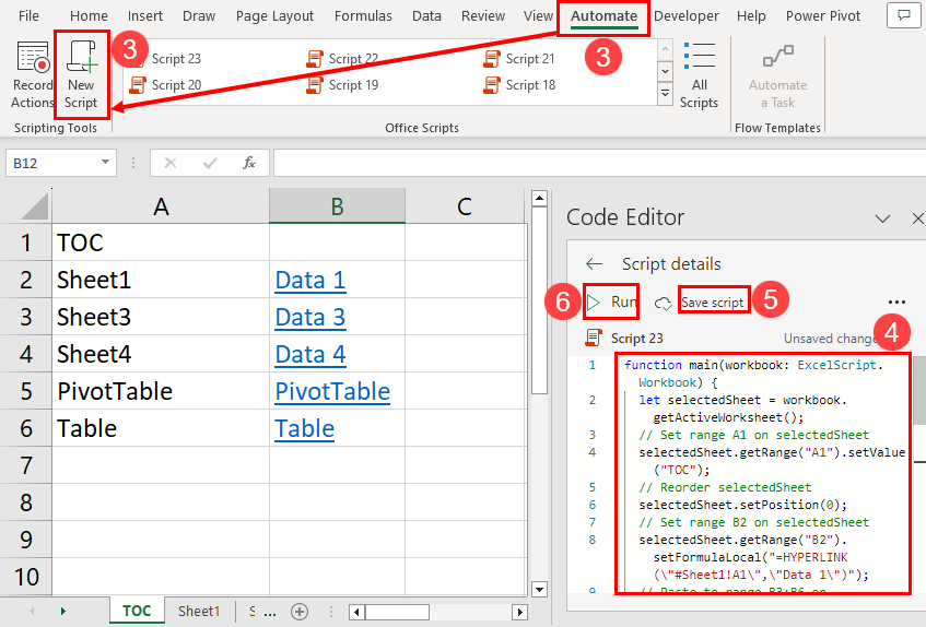
  function main(workbook: ExcelScript.Workbook) < let selectedSheet = workbook.getActiveWorksheet(); // Set range A1 on selectedSheet selectedSheet.getRange("A1").setValue("TOC"); // Reorder selectedSheet selectedSheet.setPosition(0); // Set range B2 on selectedSheet selectedSheet.getRange("B2").setFormulaLocal("=HYPERLINK(\"#Sheet1!A1\",\"Data 1\")"); // Paste to range B3:B6 on selectedSheet from range B2 on selectedSheet selectedSheet.getRange("B3:B6").copyFrom(selectedSheet.getRange("B2"), ExcelScript.RangeCopyType.all, false, false); // Set range B3:B6 on selectedSheet selectedSheet.getRange("B3:B6").setFormulasLocal([["=HYPERLINK(\"#Sheet3!A1\",\"Data 3\")"],["=HYPERLINK(\"#Sheet4!A1\",\"Data 4\")"],["=HYPERLINK(\"#PivotTable!A1\",\"PivotTable\")"],["=HYPERLINK(\"#Table!A1\",\"Table\")"]]); // Auto fit the columns of range B:B on selectedSheet selectedSheet.getRange("B:B").getFormat().autofitColumns(); >

  1. Click the Save script option.
  2. Hit the Run button to execute the code.

  If the TOC tab on your end is exactly the same as the example in this tutorial, the script will create a table of contents with redirect links.

  Suppose your workbook is slightly different, then modify these code elements:

  • getRange("B2") should be getRange("C2") , getRange("D2") , etc., according to the first cell where you’d like to apply the first HYPERLINK function.
  • In the HYPERLINK function, modify the worksheet reference Sheet1!A1 to the exact worksheet and cell you’d like to refer to, like Sheet2!B1 , Sheet3!C1 , etc.
  • Change cell range B3:B6 to the exact cell range in the column up to which you’d like to apply the above formula. For example, E1:E100 in column E.
  • Finally, you’ll need to modify the sheet reference names in each HYPERLINK formula according to your own workbook.

  Conclusions

  So far, you learned four different methods to create an Excel table of contents. Also, these methods come with different levels of automation. Depending on the number of components in your Excel workbook, like the count of worksheets, charts, PivotTables, etc., you must choose the most appropriate method.

  When the workbook is comparatively smaller, like only a few worksheets, charts, tables, etc., you can rely on the custom function.

  If the workbook is pretty large, try the Excel VBA method. If you need to create an Excel table of contents in Excel for the web app automatically, try the Office Scripts method. You can also try the Power Query method.

  Once you’ve tried the above methods, comment below to tell us which method you liked the most.

  About the Author

  Tamal Das

  I'm a freelance writer at HowToExcel.org. After completing my MS in Science, I joined reputed IT consultancy companies to acquire hands-on knowledge of data analysis and data visualization techniques as a business analyst. Now, I'm a professional freelance content writer for everything Excel and its advanced support tools, like Power Pivot, Power Query, Office Scripts, and Excel VBA. I published many tutorials and how-to articles on Excel for sites like MakeUseOf, AddictiveTips, OnSheets, Technipages, and AppleToolBox. In weekends, I perform in-depth web search to learn the latest tricks and tips of Excel so I can write on these in the weekdays!

  Subscribe

  Subscribe for awesome Microsoft Excel videos 😃

  👉 Find out more about our Advanced Formulas course!

  Top Posts

  • Pivot Table Tips and Tricks You Need to Know
  • Everything You Need to Know About Excel Tables
  • The Complete Guide to Power Query
  • Introduction To Power Query M Code
  • The Complete List of Keyboard Shortcuts in Microsoft Excel
  • The Complete List of VBA Keyboard Shortcuts in Microsoft Excel